Getting Start with De Novo CIDER (dnCIDER)
Source:vignettes/dnCIDER_highlevel.Rmd
dnCIDER_highlevel.RmdLoad pancreas data
The example data can be downloaded from https://figshare.com/s/d5474749ca8c711cc205.
Pancreatic cell data\(^1\) contain cells from human (8241 cells) and mouse (1886 cells).
load("../data/pancreas_counts.RData") # count matrix
load("../data/pancreas_meta.RData") # meta data/cell information
seu <- CreateSeuratObject(counts = pancreas_counts, meta.data = pancreas_meta)
table(seu$Batch)
#>
#> human mouse
#>  8241  1886
Perform dnCIDER (high-level)
DnCIDER contains three steps
seu <- initialClustering(seu, additional.vars.to.regress = "Sample", dims = 1:15)
#>
  |
  |                                                                      |   0%
  |
  |===================================                                   |  50%
  |
  |======================================================================| 100%
ider <- getIDEr(seu, downsampling.size = 35, use.parallel = FALSE, verbose = FALSE)
seu <- finalClustering(seu, ider, cutree.h = 0.35) # final clustering
Visualise clustering results
We use the Seurat pipeline to perform normalisation
(NormalizeData), preprocessing
(FindVariableFeatures and ScaleData) and
dimension reduction (RunPCA and RunTSNE).
seu <- NormalizeData(seu, verbose = FALSE)
seu <- FindVariableFeatures(seu, selection.method = "vst", nfeatures = 2000, verbose = FALSE)
seu <- ScaleData(seu, verbose = FALSE)
seu <- RunPCA(seu, npcs = 20, verbose = FALSE)
seu <- RunTSNE(seu, reduction = "pca", dims = 1:12)
We can see
scatterPlot(seu, "tsne", colour.by = "CIDER_cluster", title = "asCIDER clustering results") 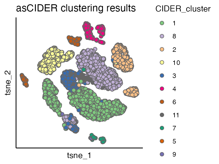
By comparing the dnCIDER results to the cell annotation from the publication\(^1\), we observe that dnCIDER correctly identify the majority of populations across two species.
scatterPlot(seu, "tsne", colour.by = "Group", title = "Ground truth of cell populations") 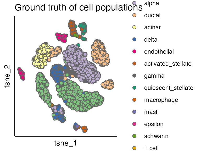
Technical
sessionInfo()
#> R version 4.1.2 (2021-11-01)
#> Platform: x86_64-apple-darwin17.0 (64-bit)
#> Running under: macOS Big Sur 10.16
#>
#> Matrix products: default
#> BLAS:   /Library/Frameworks/R.framework/Versions/4.1/Resources/lib/libRblas.0.dylib
#> LAPACK: /Library/Frameworks/R.framework/Versions/4.1/Resources/lib/libRlapack.dylib
#>
#> locale:
#> [1] en_US.UTF-8/en_US.UTF-8/en_US.UTF-8/C/en_US.UTF-8/en_US.UTF-8
#>
#> attached base packages:
#> [1] parallel  stats     graphics  grDevices utils     datasets  methods
#> [8] base
#>
#> other attached packages:
#> [1] cowplot_1.1.1      SeuratObject_4.0.4 Seurat_4.1.0       CIDER_0.99.1
#>
#> loaded via a namespace (and not attached):
#>   [1] systemfonts_1.0.2     plyr_1.8.6            igraph_1.2.8
#>   [4] lazyeval_0.2.2        splines_4.1.2         listenv_0.8.0
#>   [7] scattermore_0.7       ggplot2_3.4.2         digest_0.6.28
#>  [10] foreach_1.5.1         htmltools_0.5.2       viridis_0.6.2
#>  [13] fansi_0.5.0           magrittr_2.0.1        memoise_2.0.0
#>  [16] tensor_1.5            cluster_2.1.2         doParallel_1.0.16
#>  [19] ROCR_1.0-11           limma_3.50.0          globals_0.16.1
#>  [22] matrixStats_0.61.0    pkgdown_2.0.7         spatstat.sparse_2.0-0
#>  [25] colorspace_2.0-2      ggrepel_0.9.3         textshaping_0.3.6
#>  [28] xfun_0.28             dplyr_1.1.2           crayon_1.5.2
#>  [31] jsonlite_1.7.2        spatstat.data_2.1-0   survival_3.2-13
#>  [34] zoo_1.8-9             iterators_1.0.13      glue_1.6.2
#>  [37] polyclip_1.10-0       gtable_0.3.0          leiden_0.3.9
#>  [40] kernlab_0.9-29        future.apply_1.8.1    abind_1.4-5
#>  [43] scales_1.2.1          pheatmap_1.0.12       DBI_1.1.1
#>  [46] edgeR_3.36.0          miniUI_0.1.1.1        Rcpp_1.0.7
#>  [49] viridisLite_0.4.0     xtable_1.8-4          reticulate_1.22
#>  [52] spatstat.core_2.3-1   htmlwidgets_1.5.4     httr_1.4.2
#>  [55] RColorBrewer_1.1-2    ellipsis_0.3.2        ica_1.0-2
#>  [58] farver_2.1.0          pkgconfig_2.0.3       sass_0.4.0
#>  [61] uwot_0.1.10           deldir_1.0-6          locfit_1.5-9.4
#>  [64] utf8_1.2.2            tidyselect_1.2.0      labeling_0.4.2
#>  [67] rlang_1.1.1           reshape2_1.4.4        later_1.3.0
#>  [70] munsell_0.5.0         tools_4.1.2           cachem_1.0.6
#>  [73] cli_3.4.1             dbscan_1.1-8          generics_0.1.1
#>  [76] ggridges_0.5.3        evaluate_0.14         stringr_1.5.0
#>  [79] fastmap_1.1.0         yaml_2.2.1            ragg_1.1.3
#>  [82] goftest_1.2-3         knitr_1.36            fs_1.5.0
#>  [85] fitdistrplus_1.1-6    purrr_1.0.1           RANN_2.6.1
#>  [88] pbapply_1.5-0         future_1.28.0         nlme_3.1-153
#>  [91] mime_0.12             compiler_4.1.2        rstudioapi_0.13
#>  [94] plotly_4.10.0         png_0.1-7             spatstat.utils_2.2-0
#>  [97] tibble_3.2.1          bslib_0.3.1           stringi_1.7.5
#> [100] highr_0.9             desc_1.4.0            lattice_0.20-45
#> [103] Matrix_1.3-4          vctrs_0.6.2           pillar_1.9.0
#> [106] lifecycle_1.0.3       spatstat.geom_2.4-0   lmtest_0.9-39
#> [109] jquerylib_0.1.4       RcppAnnoy_0.0.19      data.table_1.14.2
#> [112] irlba_2.3.3           httpuv_1.6.3          patchwork_1.1.1
#> [115] R6_2.5.1              promises_1.2.0.1      KernSmooth_2.23-20
#> [118] gridExtra_2.3         parallelly_1.32.1     codetools_0.2-18
#> [121] MASS_7.3-54           rprojroot_2.0.2       withr_2.5.0
#> [124] sctransform_0.3.3     mgcv_1.8-38           grid_4.1.2
#> [127] rpart_4.1-15          tidyr_1.3.0           rmarkdown_2.11
#> [130] Rtsne_0.15            shiny_1.7.1