Detailed walk-through of de novo CIDER (dnCIDER) on pancreas data
Source:vignettes/dnCIDER.Rmd
dnCIDER.RmdIntroduction
This vignette performs dnCIDER on a cross-species pancreas dataset. It is aimed to show the underneath structure of dnCIDER compared to the other high level vignette.
Load example data
The example data can be downloaded from https://figshare.com/s/d5474749ca8c711cc205.
Pancreatic cell data\(^1\) contain cells from human (8241 cells) and mouse (1886 cells).
load("../data/pancreas_counts.RData") # count matrix
load("../data/pancreas_meta.RData") # meta data/cell information
seu <- CreateSeuratObject(counts = pancreas_counts, meta.data = pancreas_meta)
table(seu$Batch)
#>
#> human mouse
#>  8241  1886
Perform initial clustering
seu_list <- Seurat::SplitObject(seu, split.by = "Batch")
seu_list <- mclapply(seu_list, function(x) {
  x <- NormalizeData(x, normalization.method = "LogNormalize",
                     scale.factor = 10000, verbose = FALSE)
  x <- FindVariableFeatures(x, selection.method = "vst",
                            nfeatures = 2000, verbose = FALSE)
  x <- ScaleData(x, verbose = FALSE, vars.to.regress = "Sample")
  x <- RunPCA(x, features = VariableFeatures(object = x), verbose = FALSE)
  x <- FindNeighbors(x, dims = 1:15, verbose = FALSE)
  x <- FindClusters(x, resolution = 0.6, verbose = FALSE)
  return(x)
})| 0 | 1 | 2 | 3 | 4 | 5 | 6 | 7 | 8 | 9 | 10 | 11 | 12 | 13 | 14 | 15 | 16 | 17 | 18 | |
|---|---|---|---|---|---|---|---|---|---|---|---|---|---|---|---|---|---|---|---|
| acinar | 0 | 0 | 823 | 0 | 0 | 0 | 1 | 1 | 2 | 102 | 0 | 0 | 0 | 0 | 0 | 0 | 0 | 3 | 0 |
| activated_stellate | 0 | 0 | 0 | 1 | 0 | 0 | 0 | 0 | 269 | 0 | 0 | 0 | 0 | 0 | 0 | 0 | 1 | 4 | 0 |
| alpha | 1067 | 3 | 0 | 0 | 0 | 665 | 0 | 0 | 0 | 0 | 251 | 243 | 1 | 6 | 0 | 0 | 1 | 0 | 4 |
| b_cell | 0 | 0 | 0 | 0 | 0 | 0 | 0 | 0 | 0 | 0 | 0 | 0 | 0 | 0 | 0 | 0 | 0 | 0 | 0 |
| beta | 1 | 886 | 2 | 812 | 740 | 1 | 0 | 0 | 0 | 0 | 2 | 0 | 3 | 2 | 1 | 0 | 4 | 0 | 1 |
| delta | 0 | 3 | 2 | 1 | 3 | 0 | 0 | 0 | 0 | 0 | 1 | 0 | 215 | 1 | 216 | 0 | 148 | 0 | 2 |
| ductal | 1 | 1 | 6 | 0 | 0 | 0 | 469 | 386 | 0 | 169 | 0 | 0 | 1 | 0 | 0 | 0 | 0 | 0 | 0 |
| endothelial | 0 | 0 | 0 | 0 | 0 | 0 | 0 | 0 | 1 | 0 | 0 | 0 | 0 | 0 | 0 | 212 | 0 | 1 | 0 |
| epsilon | 0 | 0 | 0 | 0 | 0 | 0 | 0 | 0 | 0 | 0 | 0 | 0 | 8 | 8 | 0 | 0 | 1 | 0 | 0 |
| gamma | 1 | 1 | 0 | 0 | 0 | 0 | 0 | 0 | 0 | 0 | 1 | 0 | 3 | 210 | 0 | 0 | 25 | 0 | 0 |
| immune_other | 0 | 0 | 0 | 0 | 0 | 0 | 0 | 0 | 0 | 0 | 0 | 0 | 0 | 0 | 0 | 0 | 0 | 0 | 0 |
| macrophage | 0 | 0 | 0 | 0 | 0 | 0 | 0 | 0 | 0 | 0 | 0 | 0 | 0 | 0 | 0 | 0 | 0 | 0 | 39 |
| mast | 0 | 0 | 0 | 0 | 0 | 0 | 0 | 0 | 0 | 0 | 0 | 0 | 0 | 0 | 0 | 0 | 0 | 0 | 25 |
| quiescent_stellate | 1 | 0 | 0 | 1 | 0 | 0 | 1 | 0 | 4 | 0 | 0 | 0 | 0 | 0 | 0 | 0 | 0 | 153 | 0 |
| schwann | 0 | 0 | 0 | 0 | 0 | 0 | 0 | 0 | 10 | 0 | 0 | 0 | 0 | 0 | 0 | 0 | 0 | 0 | 0 |
| t_cell | 0 | 0 | 0 | 0 | 0 | 0 | 0 | 0 | 0 | 0 | 0 | 0 | 0 | 0 | 0 | 0 | 0 | 0 | 7 |
seu_list <- mclapply(seu_list, RunTSNE, dims = 1:15)
p1 <- scatterPlot(seu_list[[1]], "tsne", colour.by = "seurat_clusters")
p2 <- scatterPlot(seu_list[[2]], "tsne", colour.by = "seurat_clusters")
cowplot::plot_grid(p1,p2)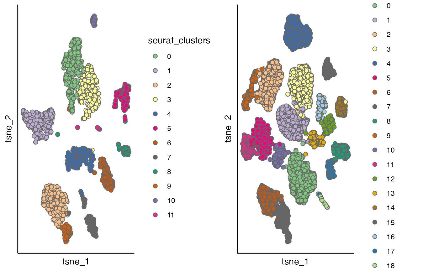
dist_coef <- getDistMat(seu_list, downsampling.size = 50)
#>
  |
  |                                                                      |   0%
  |
  |===================================                                   |  50%
  |
  |======================================================================| 100%
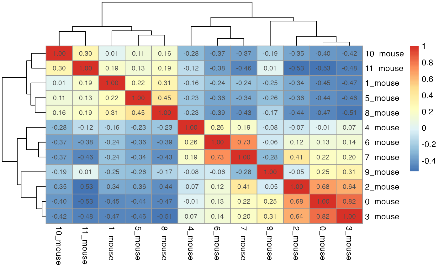
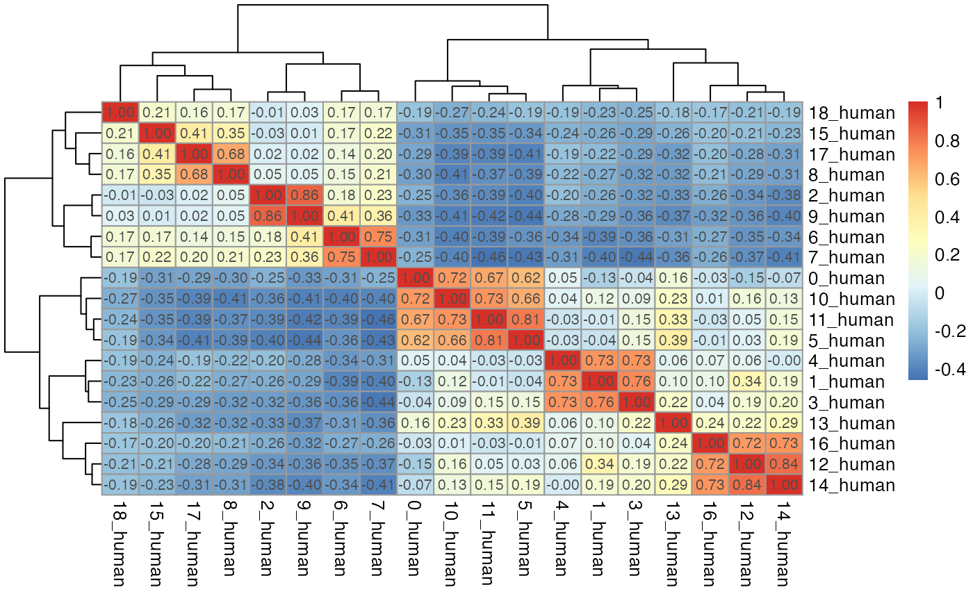
par(mfrow = c(length(seu_list),1))
for(i in which(sapply(dist_coef, function(x) return(!is.null(x))))){
  tmp <- dist_coef[[i]] + t(dist_coef[[i]])
  diag(tmp) <- 1
  pheatmap::pheatmap(tmp, display_numbers = TRUE)
}
for(seu_itor in 1:2){
  tmp <- dist_coef[[seu_itor]] + t(dist_coef[[seu_itor]])
  diag(tmp) <- 1
  tmp <- 1 - tmp
  hc <- hclust(as.dist(tmp), method = "average")
  hres <- cutree(hc, h = 0.4)
  df_hres <- data.frame(hres)
  df_hres$hres <- paste0(df_hres$hres, "_", unique(seu_list[[seu_itor]]$Batch))
  seu_list[[seu_itor]]$inicluster_tmp <- paste0(seu_list[[seu_itor]]$seurat_clusters, "_", seu_list[[seu_itor]]$Batch)
  seu_list[[seu_itor]]$inicluster <- df_hres$hres[match(seu_list[[seu_itor]]$inicluster_tmp,rownames(df_hres))]
}
# plot(as.dendrogram(hc), horiz = T)
p1 <- scatterPlot(seu_list[[1]], "tsne", "inicluster")
p2 <- scatterPlot(seu_list[[2]], "tsne", "inicluster")
plot_grid(p1,p2)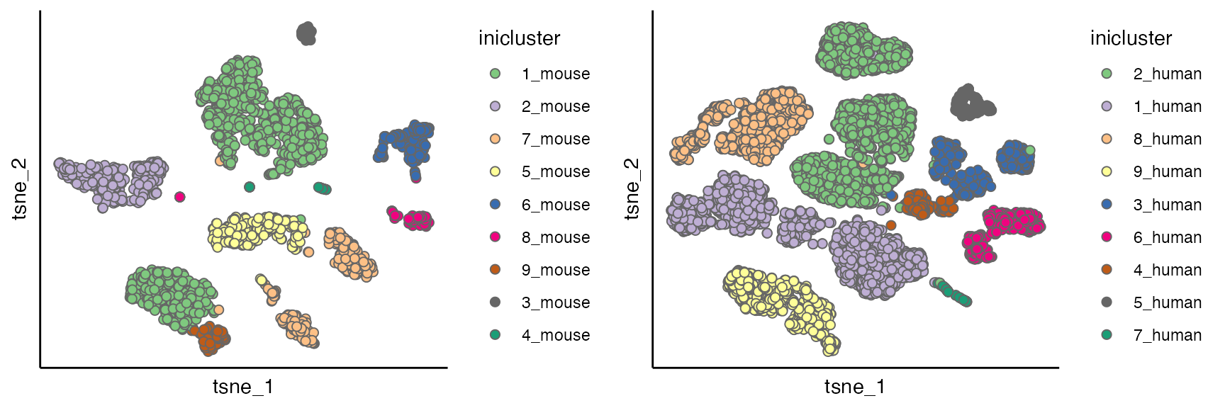
scatterPlot(seu_list[[2]], "tsne", "Group")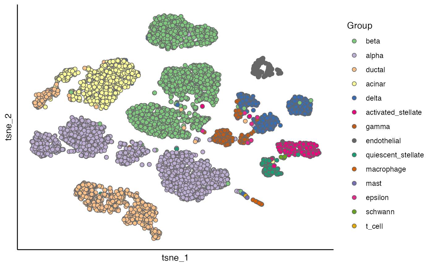
Calculate of IDER similarity matrix
res <- unlist(lapply(seu_list, function(x) return(x$inicluster)))
res_names <- unlist(lapply(seu_list, function(x) return(colnames(x))))
seu$initial_cluster <- res[match(colnames(seu), res_names)]

ider <- getIDEr(seu,
                group.by.var = "initial_cluster",
                batch.by.var = "Batch",
                downsampling.size = 35,
                use.parallel = FALSE, verbose = FALSE)
net <- plotNetwork(seu, ider, colour.by = "Group" , vertex.size = 0.6, weight.factor = 5)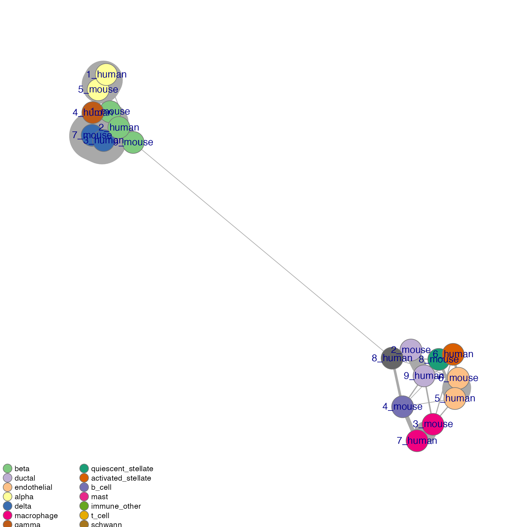
hc <- hclust(as.dist(1-(ider[[1]] + t(ider[[1]])))/2)
plot(as.dendrogram(hc), horiz = TRUE)
Perform final Clustering
seu <- finalClustering(seu, ider, cutree.h = 0.35) # final clustering
seu <- NormalizeData(seu, verbose = FALSE)
seu <- FindVariableFeatures(seu, selection.method = "vst",
                            nfeatures = 2000, verbose = FALSE)
seu <- ScaleData(seu, verbose = FALSE)
seu <- RunPCA(seu, npcs = 20, verbose = FALSE)
seu <- RunTSNE(seu, reduction = "pca", dims = 1:12)
plot_list <- list()
plot_list[[1]] <- scatterPlot(seu, "tsne", colour.by = "CIDER_cluster", title = "asCIDER clustering results")
plot_list[[2]] <- scatterPlot(seu, "tsne", colour.by = "Group", title = "Ground truth of cell populations")
plot_grid(plotlist = plot_list, ncol = 2)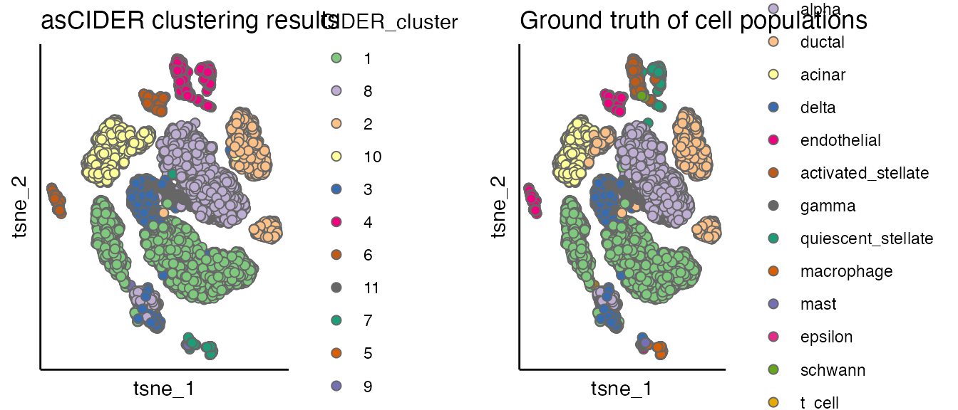
Technical
sessionInfo()
#> R version 4.1.2 (2021-11-01)
#> Platform: x86_64-apple-darwin17.0 (64-bit)
#> Running under: macOS Big Sur 10.16
#>
#> Matrix products: default
#> BLAS:   /Library/Frameworks/R.framework/Versions/4.1/Resources/lib/libRblas.0.dylib
#> LAPACK: /Library/Frameworks/R.framework/Versions/4.1/Resources/lib/libRlapack.dylib
#>
#> locale:
#> [1] en_US.UTF-8/en_US.UTF-8/en_US.UTF-8/C/en_US.UTF-8/en_US.UTF-8
#>
#> attached base packages:
#> [1] parallel  stats     graphics  grDevices utils     datasets  methods
#> [8] base
#>
#> other attached packages:
#> [1] cowplot_1.1.1      SeuratObject_4.0.4 Seurat_4.1.0       CIDER_0.99.1
#>
#> loaded via a namespace (and not attached):
#>   [1] systemfonts_1.0.2     plyr_1.8.6            igraph_1.2.8
#>   [4] lazyeval_0.2.2        splines_4.1.2         listenv_0.8.0
#>   [7] scattermore_0.7       ggplot2_3.4.2         digest_0.6.28
#>  [10] foreach_1.5.1         htmltools_0.5.2       viridis_0.6.2
#>  [13] fansi_0.5.0           magrittr_2.0.1        memoise_2.0.0
#>  [16] tensor_1.5            cluster_2.1.2         doParallel_1.0.16
#>  [19] ROCR_1.0-11           limma_3.50.0          globals_0.16.1
#>  [22] matrixStats_0.61.0    pkgdown_2.0.7         spatstat.sparse_2.0-0
#>  [25] colorspace_2.0-2      ggrepel_0.9.3         textshaping_0.3.6
#>  [28] xfun_0.28             dplyr_1.1.2           crayon_1.5.2
#>  [31] jsonlite_1.7.2        spatstat.data_2.1-0   survival_3.2-13
#>  [34] zoo_1.8-9             iterators_1.0.13      glue_1.6.2
#>  [37] polyclip_1.10-0       gtable_0.3.0          leiden_0.3.9
#>  [40] kernlab_0.9-29        future.apply_1.8.1    abind_1.4-5
#>  [43] scales_1.2.1          pheatmap_1.0.12       DBI_1.1.1
#>  [46] edgeR_3.36.0          miniUI_0.1.1.1        Rcpp_1.0.7
#>  [49] viridisLite_0.4.0     xtable_1.8-4          reticulate_1.22
#>  [52] spatstat.core_2.3-1   htmlwidgets_1.5.4     httr_1.4.2
#>  [55] RColorBrewer_1.1-2    ellipsis_0.3.2        ica_1.0-2
#>  [58] farver_2.1.0          pkgconfig_2.0.3       sass_0.4.0
#>  [61] uwot_0.1.10           deldir_1.0-6          locfit_1.5-9.4
#>  [64] utf8_1.2.2            labeling_0.4.2        tidyselect_1.2.0
#>  [67] rlang_1.1.1           reshape2_1.4.4        later_1.3.0
#>  [70] munsell_0.5.0         tools_4.1.2           cachem_1.0.6
#>  [73] cli_3.4.1             dbscan_1.1-8          generics_0.1.1
#>  [76] ggridges_0.5.3        evaluate_0.14         stringr_1.5.0
#>  [79] fastmap_1.1.0         yaml_2.2.1            ragg_1.1.3
#>  [82] goftest_1.2-3         knitr_1.36            fs_1.5.0
#>  [85] fitdistrplus_1.1-6    purrr_1.0.1           RANN_2.6.1
#>  [88] pbapply_1.5-0         future_1.28.0         nlme_3.1-153
#>  [91] mime_0.12             compiler_4.1.2        rstudioapi_0.13
#>  [94] plotly_4.10.0         png_0.1-7             spatstat.utils_2.2-0
#>  [97] tibble_3.2.1          bslib_0.3.1           stringi_1.7.5
#> [100] highr_0.9             desc_1.4.0            lattice_0.20-45
#> [103] Matrix_1.3-4          vctrs_0.6.2           pillar_1.9.0
#> [106] lifecycle_1.0.3       spatstat.geom_2.4-0   lmtest_0.9-39
#> [109] jquerylib_0.1.4       RcppAnnoy_0.0.19      data.table_1.14.2
#> [112] irlba_2.3.3           httpuv_1.6.3          patchwork_1.1.1
#> [115] R6_2.5.1              promises_1.2.0.1      KernSmooth_2.23-20
#> [118] gridExtra_2.3         parallelly_1.32.1     codetools_0.2-18
#> [121] MASS_7.3-54           rprojroot_2.0.2       withr_2.5.0
#> [124] sctransform_0.3.3     mgcv_1.8-38           grid_4.1.2
#> [127] rpart_4.1-15          tidyr_1.3.0           rmarkdown_2.11
#> [130] Rtsne_0.15            shiny_1.7.1