Introduction
This vignette performs asCIDER, a meta-clustering method, on a cross-species pancreas dataset. AsCIDER is aimed to achieve the clustering task in data confounded by unwanted variables. In this scenario, the unwanted variable is species effects.
asCIDER is short for assisted CIDER, assisted by the prior batch-specific annotations or clustering results.
Pancreas data
The example data can be downloaded from https://figshare.com/s/d5474749ca8c711cc205.
This data\(^1\) contain cells from human (8241 cells) and mouse (1886 cells).
load("../data/pancreas_counts.RData") # count matrix
load("../data/pancreas_meta.RData") # meta data/cell information
seu <- CreateSeuratObject(counts = pancreas_counts, meta.data = pancreas_meta)
table(seu$Batch)
#>
#> human mouse
#>  8241  1886
Exam if data are confounded
Prior to use CIDER (or other integration methods for clustering) it is important to exam if clustering will be confounded by the cross-species factors.
Her we first perform the conventional Seurat\(^2\) clustering pipeline.
seu <- NormalizeData(seu, verbose = FALSE)
seu <- FindVariableFeatures(seu, selection.method = "vst", nfeatures = 2000, verbose = FALSE)
seu <- ScaleData(seu, verbose = FALSE)
seu <- RunPCA(seu, npcs = 20, verbose = FALSE)
seu <- RunTSNE(seu, reduction = "pca", dims = 1:12)
Confounded dimension reduction
The PCA and t-SNE plots both showed that the data are confounded by species.
The scatterPlot function is used to generate dimension
reduction figures. It takes input of a Seurat object (seu
here), the name of reduction (pca and tsne
here), the variable deciding dot colours (Batch here) and
the title of plots. See more information by
?scatterPlot
p1 <- scatterPlot(seu, "pca",colour.by = "Batch", title = "PCA")
p2 <- scatterPlot(seu, "tsne",colour.by = "Batch", title = "t-SNE")
plot_grid(p1, p2)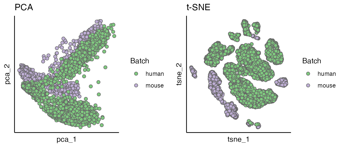
Confounded clustering results
seu <- FindNeighbors(seu, dims = 1:12)
#> Computing nearest neighbor graph
#> Computing SNN
seu <- FindClusters(seu)
#> Modularity Optimizer version 1.3.0 by Ludo Waltman and Nees Jan van Eck
#>
#> Number of nodes: 10127
#> Number of edges: 352494
#>
#> Running Louvain algorithm...
#> Maximum modularity in 10 random starts: 0.9149
#> Number of communities: 22
#> Elapsed time: 1 seconds

scatterPlot(seu, "tsne",colour.by = "seurat_clusters", title = "t-SNE") 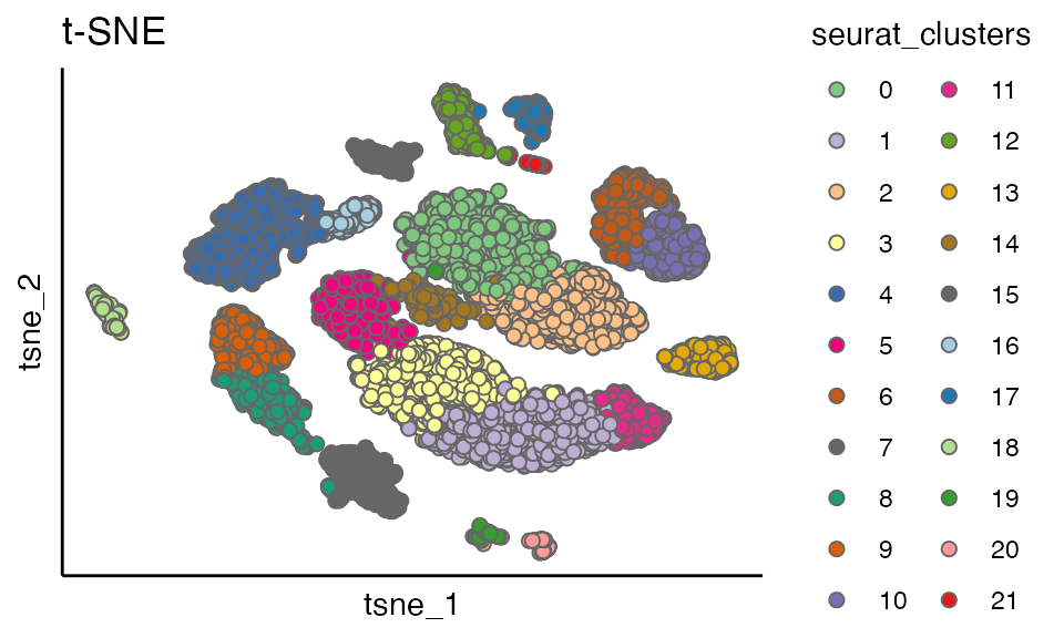
res <- data.frame(table(seu$seurat_clusters, seu$Batch))
ggplot(res, aes(fill=Var2, y=Freq, x=Var1)) +
    geom_bar(position="stack", stat="identity") + xlab("CIDER_cluster") + ylab("Proportions")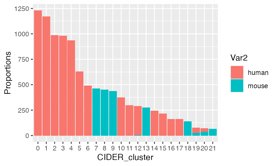
asCIDER
Prepare initial clusters
asCIDER uses existing within-batch clustering results. Here we concatenate the batch ID and the within-batch cluster ID to obtain cluster-specific groups (i.e. initial clusters).
seu$initial_cluster <- paste(seu$Group, seu$Batch, sep = "_")
table(seu$initial_cluster)
#>
#>             acinar_human activated_stellate_human activated_stellate_mouse
#>                      932                      275                       14
#>              alpha_human              alpha_mouse             b_cell_mouse
#>                     2241                      191                       10
#>               beta_human               beta_mouse              delta_human
#>                     2455                      894                      592
#>              delta_mouse             ductal_human             ductal_mouse
#>                      218                     1033                      275
#>        endothelial_human        endothelial_mouse            epsilon_human
#>                      214                      139                       17
#>              gamma_human              gamma_mouse       immune_other_mouse
#>                      241                       41                        8
#>         macrophage_human         macrophage_mouse               mast_human
#>                       39                       36                       25
#> quiescent_stellate_human quiescent_stellate_mouse            schwann_human
#>                      160                       47                       10
#>            schwann_mouse             t_cell_human             t_cell_mouse
#>                        6                        7                        7
Calculate of IDER similarity matrix
The function getIDEr calculate the IDER-based distance
matrix.
By default, it will use the column called “initial_cluster” as initial clusters, and “Batch” as batch. If you are using columns other than this two, please revise these two parameters.
For this step, you can choose to use parallel computation by setting
use.parallel = TRUE or not (default
use.parallel = FALSE). The default number of cores used for
parallel computation is
detectCores(logical = FALSE) - 1.
ider <- getIDEr(seu,
group.by.var = "initial_cluster",
batch.by.var = "Batch",
downsampling.size = 35,
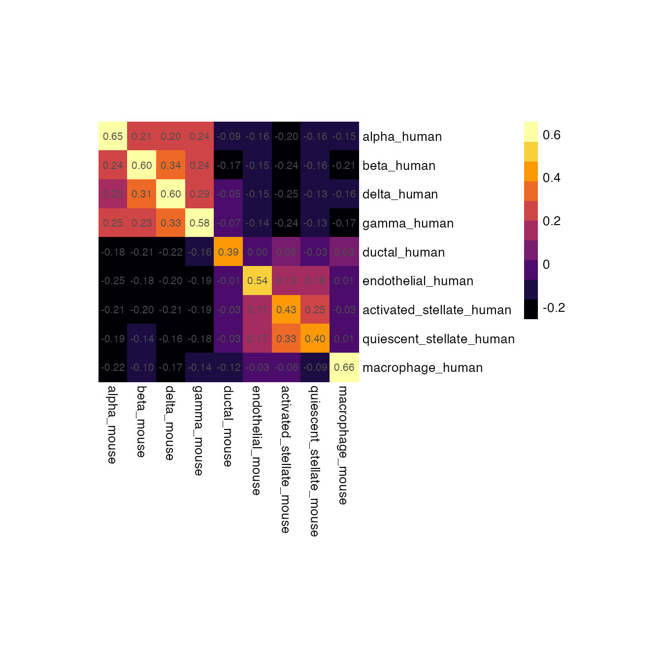
use.parallel = FALSE, verbose = FALSE)Visualise the similarity matrix
groups <- c("alpha","beta","delta", "gamma","ductal","endothelial", "activated_stellate", "quiescent_stellate", "macrophage")
idx1 <- paste0(groups, "_human")
idx2 <- paste0(groups, "_mouse")

pheatmap::pheatmap(
  ider[[1]][idx1, idx2],
  color = inferno(10),
  border_color = NA,
  display_numbers = TRUE,
  cluster_rows = FALSE,
  cluster_cols = FALSE,
  width = 7,
  height = 5,
  cellwidth = 22,
  cellheight = 22
)
Perform final Clustering
Next we put both Seurat object and the similarity matrix list into
finalClustering. You can either cut trees by height (set
cutree.by = 'h) or by k (set cutree.by = 'k).
The default is cutting by the height of 0.45.
The final clustering results are stored in Colume
cider_final_cluster of Seurat object metadata and can be
extracted using seu$cider_final_cluster.
seu <- finalClustering(seu, ider, cutree.h = 0.45)
head(seu@meta.data)
#>                             orig.ident nCount_RNA nFeature_RNA Batch   Group
#> mouse1_lib1.final_cell_0001     mouse1      11003         2994 mouse    beta
#> mouse1_lib1.final_cell_0002     mouse1      10701         3565 mouse  ductal
#> mouse1_lib1.final_cell_0003     mouse1       9445         2401 mouse   delta
#> mouse1_lib1.final_cell_0004     mouse1       8193         2865 mouse schwann
#> mouse1_lib1.final_cell_0005     mouse1       7323         2355 mouse   delta
#> mouse1_lib1.final_cell_0006     mouse1       8504         2637 mouse    beta
#>                             Sample RNA_snn_res.0.8 seurat_clusters
#> mouse1_lib1.final_cell_0001 mouse1               9               9
#> mouse1_lib1.final_cell_0002 mouse1              13              13
#> mouse1_lib1.final_cell_0003 mouse1               7               7
#> mouse1_lib1.final_cell_0004 mouse1              21              21
#> mouse1_lib1.final_cell_0005 mouse1               7               7
#> mouse1_lib1.final_cell_0006 mouse1               8               8
#>                             initial_cluster CIDER_cluster
#> mouse1_lib1.final_cell_0001      beta_mouse             1
#> mouse1_lib1.final_cell_0002    ductal_mouse             2
#> mouse1_lib1.final_cell_0003     delta_mouse             3
#> mouse1_lib1.final_cell_0004   schwann_mouse             4
#> mouse1_lib1.final_cell_0005     delta_mouse             3
#> mouse1_lib1.final_cell_0006      beta_mouse             1
Visualise clustering results
plot_list <- list()
plot_list[[1]] <- scatterPlot(seu, "tsne", colour.by = "CIDER_cluster", title = "asCIDER clustering results")
plot_list[[2]] <- scatterPlot(seu, "tsne", colour.by = "Group", title = "Ground truth of cell populations")
plot_grid(plotlist = plot_list, ncol = 2)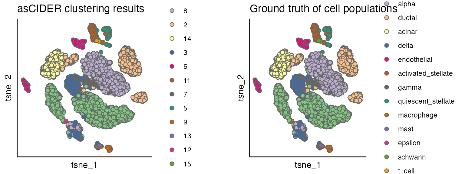
res <- data.frame(table(seu$CIDER_cluster, seu$Batch))
ggplot(res, aes(fill=Var2, y=Freq, x=Var1)) +
    geom_bar(position="stack", stat="identity") + xlab("CIDER_cluster") + ylab("Proportions")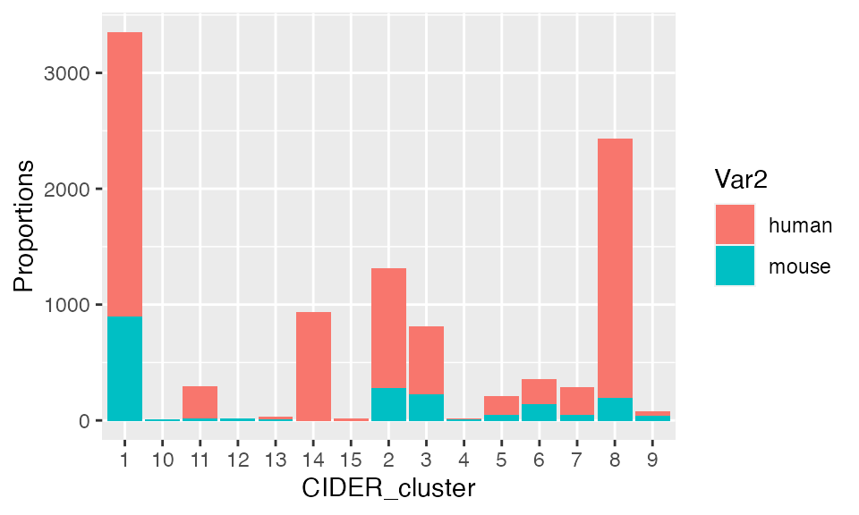
Technical
sessionInfo()
#> R version 4.1.2 (2021-11-01)
#> Platform: x86_64-apple-darwin17.0 (64-bit)
#> Running under: macOS Big Sur 10.16
#>
#> Matrix products: default
#> BLAS:   /Library/Frameworks/R.framework/Versions/4.1/Resources/lib/libRblas.0.dylib
#> LAPACK: /Library/Frameworks/R.framework/Versions/4.1/Resources/lib/libRlapack.dylib
#>
#> locale:
#> [1] en_US.UTF-8/en_US.UTF-8/en_US.UTF-8/C/en_US.UTF-8/en_US.UTF-8
#>
#> attached base packages:
#> [1] stats     graphics  grDevices utils     datasets  methods   base
#>
#> other attached packages:
#> [1] viridis_0.6.2      viridisLite_0.4.0  cowplot_1.1.1      ggplot2_3.4.2
#> [5] pheatmap_1.0.12    SeuratObject_4.0.4 Seurat_4.1.0       CIDER_0.99.1
#>
#> loaded via a namespace (and not attached):
#>   [1] systemfonts_1.0.2     plyr_1.8.6            igraph_1.2.8
#>   [4] lazyeval_0.2.2        splines_4.1.2         listenv_0.8.0
#>   [7] scattermore_0.7       digest_0.6.28         foreach_1.5.1
#>  [10] htmltools_0.5.2       fansi_0.5.0           magrittr_2.0.1
#>  [13] memoise_2.0.0         tensor_1.5            cluster_2.1.2
#>  [16] doParallel_1.0.16     ROCR_1.0-11           limma_3.50.0
#>  [19] globals_0.16.1        matrixStats_0.61.0    pkgdown_2.0.7
#>  [22] spatstat.sparse_2.0-0 colorspace_2.0-2      ggrepel_0.9.3
#>  [25] textshaping_0.3.6     xfun_0.28             dplyr_1.1.2
#>  [28] crayon_1.5.2          jsonlite_1.7.2        spatstat.data_2.1-0
#>  [31] survival_3.2-13       zoo_1.8-9             iterators_1.0.13
#>  [34] glue_1.6.2            polyclip_1.10-0       gtable_0.3.0
#>  [37] leiden_0.3.9          kernlab_0.9-29        future.apply_1.8.1
#>  [40] abind_1.4-5           scales_1.2.1          DBI_1.1.1
#>  [43] edgeR_3.36.0          miniUI_0.1.1.1        Rcpp_1.0.7
#>  [46] xtable_1.8-4          reticulate_1.22       spatstat.core_2.3-1
#>  [49] htmlwidgets_1.5.4     httr_1.4.2            RColorBrewer_1.1-2
#>  [52] ellipsis_0.3.2        ica_1.0-2             farver_2.1.0
#>  [55] pkgconfig_2.0.3       sass_0.4.0            uwot_0.1.10
#>  [58] deldir_1.0-6          locfit_1.5-9.4        utf8_1.2.2
#>  [61] tidyselect_1.2.0      labeling_0.4.2        rlang_1.1.1
#>  [64] reshape2_1.4.4        later_1.3.0           munsell_0.5.0
#>  [67] tools_4.1.2           cachem_1.0.6          cli_3.4.1
#>  [70] dbscan_1.1-8          generics_0.1.1        ggridges_0.5.3
#>  [73] evaluate_0.14         stringr_1.5.0         fastmap_1.1.0
#>  [76] yaml_2.2.1            ragg_1.1.3            goftest_1.2-3
#>  [79] knitr_1.36            fs_1.5.0              fitdistrplus_1.1-6
#>  [82] purrr_1.0.1           RANN_2.6.1            pbapply_1.5-0
#>  [85] future_1.28.0         nlme_3.1-153          mime_0.12
#>  [88] compiler_4.1.2        rstudioapi_0.13       plotly_4.10.0
#>  [91] png_0.1-7             spatstat.utils_2.2-0  tibble_3.2.1
#>  [94] bslib_0.3.1           stringi_1.7.5         highr_0.9
#>  [97] desc_1.4.0            lattice_0.20-45       Matrix_1.3-4
#> [100] vctrs_0.6.2           pillar_1.9.0          lifecycle_1.0.3
#> [103] spatstat.geom_2.4-0   lmtest_0.9-39         jquerylib_0.1.4
#> [106] RcppAnnoy_0.0.19      data.table_1.14.2     irlba_2.3.3
#> [109] httpuv_1.6.3          patchwork_1.1.1       R6_2.5.1
#> [112] promises_1.2.0.1      KernSmooth_2.23-20    gridExtra_2.3
#> [115] parallelly_1.32.1     codetools_0.2-18      MASS_7.3-54
#> [118] rprojroot_2.0.2       withr_2.5.0           sctransform_0.3.3
#> [121] mgcv_1.8-38           parallel_4.1.2        grid_4.1.2
#> [124] rpart_4.1-15          tidyr_1.3.0           rmarkdown_2.11
#> [127] Rtsne_0.15            shiny_1.7.1